Introduction
This is a (incomplete) list of potential use cases of this software. This document show what functions are required at minimum to build a valid CLUMondo model of a certain setup.
In this document you will first find an overview of the example data used to build the use cases and scenarios. Then, use cases are sorted by complexity and grouped by the involved land systems and the demands according to which the systems will be modified. The first group has use cases that can be run on two land systems and one demand. The second group is extension of this and includes additionally a third land system, but still only one demand. The third group is again an extension of the previous group and finally includes additionally a second demand. At the end of the document, there are examples that show more complex use cases.
There is a little note: Since CLUE can be and is used in various fields, we simply use the term land system or just system to denote the land surface descriptions, be they land use, land cover or any other system.
Also, this document is still work in progress (and we welcome any additions)!
Example data
Let’s first load the required packages and define the path for example data.
library(clueRIO)
#> Error in get(paste0(generic, ".", class), envir = get_method_env()) :
#>   object 'type_sum.accel' not found
library(stringr)
library(tibble)
library(terra)
#> terra 1.8.5

data <- system.file("test_data", package = "clueRIO", mustWork = TRUE)
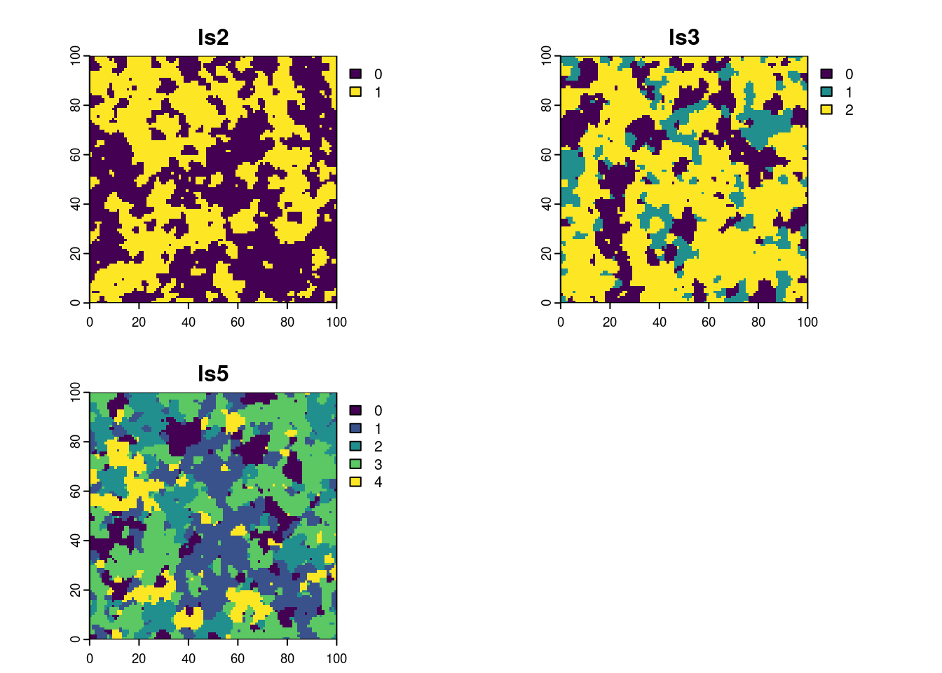
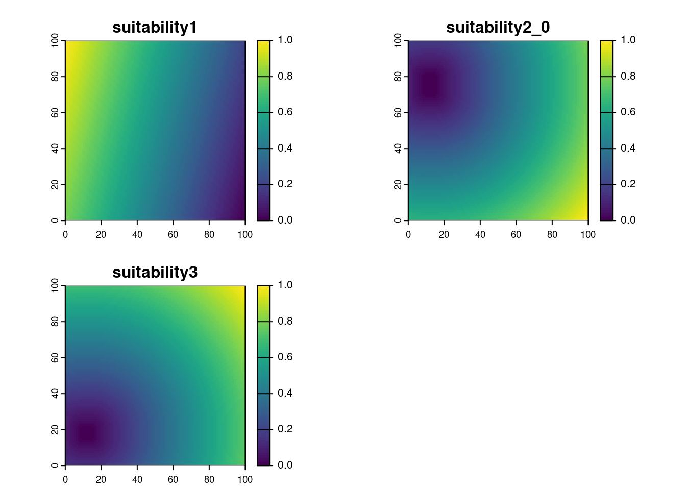
There are various tables and (highly simplified) raster layers used throughout this tutorial. Below we see, as an example, maps of land systems and suitability maps. Other data are generated with simple example code only when they are needed.
(testRast <- list.files(data, full.names = TRUE))
#> [1] "/home/runner/work/_temp/Library/clueRIO/test_data/ls2.tif"
#> [2] "/home/runner/work/_temp/Library/clueRIO/test_data/ls3.tif"
#> [3] "/home/runner/work/_temp/Library/clueRIO/test_data/ls5.tif"
#> [4] "/home/runner/work/_temp/Library/clueRIO/test_data/preference1.tif"
#> [5] "/home/runner/work/_temp/Library/clueRIO/test_data/suitability1.tif"
#> [6] "/home/runner/work/_temp/Library/clueRIO/test_data/suitability2_0.tif"
#> [7] "/home/runner/work/_temp/Library/clueRIO/test_data/suitability3.tif"
#> [8] "/home/runner/work/_temp/Library/clueRIO/test_data/test_region.gpkg"

# land systems
plot(rast(testRast[str_detect(testRast, "ls")]))
# different suitability layers
plot(rast(testRast[str_detect(testRast, "suitability")]))
minimal example (ls2d1)
In a system with cropland and forest, convert forest to cropland at a rate required only by the demand of crops.
model <- "ls2d1"

scene <- clue_scene(
  root = paste0(tempdir(), "/", model),
  name = model,
  period = c(2000, 2024),
  regions = paste0(data, "/test_region.gpkg"),
  description = "this is a minimal showcase where forest is converted to cropland to produce crops.") |>
  clue_gridded(file = paste0(data, "/ls2.tif"),
               type = "initial") |>
  clue_gridded(file = paste0(data, "/suitability1.tif"),
               type = "driver",
               name = "cropland_suit") |>
  clue_gridded(file = paste0(data, "/suitability2_0.tif"),
               type = "driver",
               name = "forest_suit") |>
  clue_landtype(name = "forest",
                resistance = 0.5,
                suitability = tibble(driver = c("const", "forest_suit"),
                                     beta = c(1, 1)),
                conversion = tibble(to = "cropland",
                                    label = "intensification")) |>
  clue_landtype(name = "cropland",
                resistance = 0.5,
                suitability = tibble(driver = c("const", "cropland_suit"),
                                     beta = c(1, 1)),
                production = tibble(name = "crops",
                                    amount = 1, priority = 1)) |>
  clue_goods(name = "crops",
             demand = tibble(year = c(2000:2024),
                             region = "ravenholm",
                             amount = seq(from = 4760, to = 5000, length.out = 25))) |>
  clue_initiate()

clue_run(scene = scene, clue.exe = ...)
ls2d1, stepwise
In a system with cropland and forest, convert forest to cropland at a rate required only by the demand of crops. Here, each year is calculated step by step, allowing further modules to interact with the input data of each new time step. This is not shown here yet, but is required as a prerequisite for some of the modifiers, discussed below.
model <- "ls2d1_step"

scene <- clue_scene(
  root = paste0(tempdir(), "/", model),
  name = model,
  period = c(2000, 2024),
  regions = paste0(data, "/test_region.gpkg"),
  description = "") |>
  clue_gridded(file = paste0(data, "/ls2.tif"),
               type = "initial") |>
  clue_gridded(file = paste0(data, "/suitability1.tif"),
               type = "driver",
               name = "cropland_suit") |>
  clue_gridded(file = paste0(data, "/suitability2_0.tif"),
               type = "driver",
               name = "forest_suit") |>
  clue_landtype(name = "forest",
                resistance = 0.5,
                suitability = tibble(driver = c("const", "forest_suit"),
                                     beta = c(1, 1)),
                conversion = tibble(to = "cropland",
                                    label = "intensification")) |>
  clue_landtype(name = "cropland",
                resistance = 0.5,
                suitability = tibble(driver = c("const", "cropland_suit"),
                                     beta = c(1, 1)),
                production = tibble(name = "crops",
                                    amount = 1, priority = 1)) |>
  clue_goods(name = "crops",
             demand = tibble(year = c(2000:2024),
                             region = "ravenholm",
                             amount = seq(from = 4760, to = 5000, length.out = 25))) |>
  clue_initiate(module = "stepwise")

clue_run(scene = scene, clue.exe = ...)…
model <- "ls2d1_protected"…
model <- "ls2d1_convLimit"…
model <- "ls2d1_limit_prot"ls2d1, dynamic driver
This model has yearly suitability layers (i.e., dynamic drivers).
model <- "ls2d1_dynamic"ls2d1, location preferences
In a system with cropland and forest, convert forest to cropland at a rate required only by the demand of crops. To indicate where forest would grow preferentially, forest has a location specific preference assigned to it.
model <- "ls2d1_preferences"

scene <- clue_scene(
  root = paste0(tempdir(), "/", model),
  name = model,
  period = c(2000, 2024),
  regions = paste0(data, "/test_region.gpkg"),
  description = "") |>
  clue_gridded(file = paste0(data, "/ls2.tif"),
               type = "initial") |>
  clue_gridded(file = paste0(data, "/suitability1.tif"),
               type = "driver",
               name = "cropland_suit") |>
  clue_gridded(file = paste0(data, "/suitability2_0.tif"),
               type = "driver",
               name = "forest_suit") |>
  clue_gridded(file = paste0(data, "/preference1.tif"),
               type = "preference",
               name = "pref_forest") |>
  clue_landtype(name = "forest",
                resistance = 0.5,
                suitability = tibble(driver = c("const", "forest_suit"),
                                     beta = c(1, 1)),
                conversion = tibble(to = "cropland",
                                    label = "intensification"),
                preference = tibble(layer = "pref_forest", weight = 1)) |>
  clue_landtype(name = "cropland",
                resistance = 0.5,
                suitability = tibble(driver = c("const", "cropland_suit"),
                                     beta = c(1, 1)),
                production = tibble(name = "crops",
                                    amount = 1, priority = 1)) |>
  clue_goods(name = "crops",
             demand = tibble(year = c(2000:2024),
                             region = "ravenholm",
                             amount = seq(from = 4760, to = 5000, length.out = 25))) |>
  clue_initiate()

clue_run(scene = scene, clue.exe = ...)ls2d1 + pasture (ls3d1)
In a system with cropland, forest and pasture, convert forest to cropland at a rate required only by the demand of crops.
model <- "ls3d1"

scene <- clue_scene(
  root = paste0(tempdir(), "/", model),
  name = model,
  period = c(2000, 2024),
  regions = paste0(data, "/test_region.gpkg"),
  description = "") |>
  clue_gridded(file = paste0(data, "/ls3.tif"),
               type = "initial") |>
  clue_gridded(file = paste0(data, "/suitability1.tif"),
               type = "driver",
               name = "cropland_suit") |>
  clue_gridded(file = paste0(data, "/suitability2_0.tif"),
               type = "driver",
               name = "forest_suit") |>
  clue_gridded(file = paste0(data, "/suitability3.tif"),
               type = "driver",
               name = "pasture_suit") |>
  clue_landtype(name = "forest",
                resistance = 0.5,
                suitability = tibble(driver = c("const", "forest_suit"),
                                     beta = c(1, 1)),
                conversion = tibble(to = "cropland",
                                    label = "intensification")) |>
  clue_landtype(name = "cropland",
                resistance = 0.5,
                suitability = tibble(driver = c("const", "cropland_suit"),
                                     beta = c(1, 1)),
                production = tibble(name = "crops",
                                    amount = 1, priority = 1)) |>
  clue_landtype(name = "pasture",
                resistance = 0.5,
                suitability = tibble(driver = c("const", "pasture_suit"),
                                     beta = c(1, 1))) |>
  clue_goods(name = "crops",
             demand = tibble(year = c(2000:2024),
                             region = "ravenholm",
                             amount = seq(from = 5845, to = 6500, length.out = 25))) |>
  clue_initiate()

clue_run(scene = scene, clue.exe = ...)
ls3d1, neighborhood
…
model <- "ls3d1_neighborhood"

scene <- clue_scene(
  root = paste0(tempdir(), "/", model),
  name = model,
  period = c(2000, 2024),
  regions = paste0(data, "/test_region.gpkg"),
  description = "") |>
  clue_gridded(file = paste0(data, "/ls3.tif"),
               type = "initial") |>
  clue_gridded(file = paste0(data, "/suitability1.tif"),
               type = "driver",
               name = "cropland_suit") |>
  clue_gridded(file = paste0(data, "/suitability2_0.tif"),
               type = "driver",
               name = "forest_suit") |>
  clue_gridded(file = paste0(data, "/suitability3.tif"),
               type = "driver",
               name = "pasture_suit") |>
  clue_gridded(file = rast(matrix(1, 3, 3)),
               type = "kernel") |>
  clue_landtype(name = "forest",
                resistance = 0.5,
                suitability = tibble(driver = c("const", "forest_suit"),
                                     beta = c(1, 1)),
                conversion = tibble(to = "cropland",
                                    label = "intensification"),
                neighborhood = tibble(type = c("kernel", "weight", "const", "forest", "cropland"),
                                      beta = c(1, 0.3, 1, 0.5, 0.5))) |>
  clue_landtype(name = "cropland",
                resistance = 0.5,
                suitability = tibble(driver = c("const", "cropland_suit"),
                                     beta = c(1, 1)),
                production = tibble(name = "crops",
                                    amount = 1, priority = 1)) |>
  clue_landtype(name = "pasture",
                resistance = 0.5,
                suitability = tibble(driver = c("const", "pasture_suit"),
                                     beta = c(1, 1))) |>
  clue_goods(name = "crops",
             demand = tibble(year = c(2000:2024),
                             region = "ravenholm",
                             amount = seq(from = 5845, to = 6500, length.out = 25))) |>
  clue_initiate()

clue_run(scene = scene, clue.exe = ...)